

IMPROVING SCIENTIST PRODUCTIVITY,
ARCHITECTURE PORTABILITY, AND APPLICATION
PERFORMANCE IN PARFLOW
by
Michael Burke
A thesis
submitted in partial ful llment
of the requirements for the degree of
Master of Science in Computer Science
Boise State University
May 2020
c 2020
Michael Burke
ALL RIGHTS RESERVED
BOISE STATE UNIVERSITY GRADUATE COLLEGE
DEFENSE COMMITTEE AND FINAL READING APPROVALS
of the thesis submitted by
Michael Burke
Thesis Title: Improving Scientist Productivity, Architecture Portability, and Application Performance in ParFlow
Date of Final Oral Examination: 11th May 2020
The following individuals read and discussed the thesis submitted by student Michael Burke, and they evaluated the presentation and response to questions during the final oral examination. They found that the student passed the final oral examination.
Dr. Catherine Olschanowsky, Ph.D. Chair, Supervisory Committee
Dr. Michael Ekstrand, Ph.D. Member, Supervisory Committee
Dr. Alejandro Flores, Ph.D. Member, Supervisory Committee
The nal reading approval of the thesis was granted by Dr. Catherine Olschanowsky, Ph.D., Chair of the Supervisory Committee. The thesis was approved by the Graduate College.
ACKNOWLEDGMENTS
I am sincerely grateful to my advisor, Dr. Catherine Olschanowsky, for her support, guidance, and encouragement. She has greatly helped me develop my technical, professional, and writing skills. The many opportunities she presented to me have advanced my career to a point I previously found unimaginable, and attending conferences and workshops I would have otherwise never considered. I am additionally grateful to her for providing me with a graduate assistantship and funding me over the course of my Masters degree. I would like to thank my supervisory committee members Dr. Michael Ekstrand and Dr. Alejandro Flores for their feedback on my proposal, thesis, and oral defense. Help re ning speci c contributions with Dr. Ekstrand was very valuable. I would also like to thank Dr. Reed Maxwell at Colorado School of Mines and Dr. Laura Condon at University of Arizona. Their direct participation enabled this thesis and its research to be possible, providing valuable perspectives from a computational scientist standpoint.
ABSTRACT
Legacy scienti c applications represent signi cant investments by universities, engineers, and researchers and contain valuable implementations of key scienti c computations. Over time hardware architectures have changed. Adapting existing code to new architectures is time consuming, expensive, and increases code complexity. The increase in complexity negatively a ects the scienti c impact of the applications. There is an immediate need to reduce complexity. We propose using abstractions to manage and reduce code complexity, improving scienti c impact of applications. This thesis presents a set of abstractions targeting boundary conditions in iterative solvers. Many scientific applications represent physical phenomena as a set of partial di erential equations (PDEs). PDEs are structured around steady state and boundary condition equations, starting from initial conditions.
The proposed abstractions separate architecture specific implementation details from the primary computation. We use ParFlow to demonstrate the e ectiveness of the abstractions. ParFlow is a hydrologic and geoscience application that simulates surface and subsurface water ow. The abstractions have enabled ParFlow developers
to successfully add new boundary conditions for the first time in 15 years, and have enabled an experimental OpenMP version of ParFlow that is transparent to computational scientists. This is achieved without requiring expensive rewrites of key computations or major codebase changes; improving developer productivity, enabling hardware portability, and allowing transparent performance optimizations.
TABLE OF CONTENTS
ABSTRACT………………………………………..
LIST OF TABLES……………………………………
LIST OF FIGURES…………………………………..
LIST OF ABBREVIATIONS ……………………………
1 Introduction………………………………………
1.1 Problem Statement. . . . . . . . . . . . . . . . . . . . . . . . . . . . . . . . . . . . . . . . .
1.2 CaseStudy:ParFlow. . . . . . . . . . . . . . . . . . . . . . . . . . . . . . . . . . . . . . .
1.3 Contributions . . . . . . . . . . . . . . . . . . . . . . . . . . . . . . . . . . . . . . . . . . . . .
1.4 Organization. . . . . . . . . . . . . . . . . . . . . . . . . . . . . . . . . . . . . . . . . . . . . .
2 Background ………………………………………
2.1 ParFlow . . . . . . . . . . . . . . . . . . . . . . . . . . . . . . . . . . . . . . . . . . . . . . . . .
2.1.1 Boundary Conditions and CONUS. . . . . . . . . . . . . . . . . . . . . . .
2.2 Domain Specific Languages . . . . . . . . . . . . . . . . . . . . . . . . . . . . . . . . . .
2.2.1 Existing Par Flowe DSL. . . . . . . . . . . . . . . . . . . . . . . . . . . . . . . .
2.3 Architecture Portability . . . . . . . . . . . . . . . . . . . . . . . . . . . . . . . . . . . . .
2.3.1 Open MP. . . . . . . . . . . . . . . . . . . . . . . . . . . . . . . . . . . . . . . . . . .
2.3.2 CUDA. . . . . . . . . . . . . . . . . . . . . . . . . . . . . . . . . . . . . . . . . . . . .
3 Boundary Condition Abstractions………………………
3.1 Design and Approach. . . . . . . . . . . . . . . . . . . . . . . . . . . . . . . . . . . . . . .
3.1.1 Setting the source of Boundary Condition Values. . . . . . . . . . . .
3.1.2 Setting Data For Each Time Step. . . . . . . . . . . . . . . . . . . . . . . .
3.1.3 Performing Boundary Condition Computations . . . . . . . . . . . . .
3.2 Backend Development . . . . . . . . . . . . . . . . . . . . . . . . . . . . . . . . . . . . . .
3.2.1 Data owand Proling Analysis . . . . . . . . . . . . . . . . . . . . . . . . .
3.2.2 Open MP. . . . . . . . . . . . . . . . . . . . . . . . . . . . . . . . . . . . . . . . . . .
3.2.3 Limitations . . . . . . . . . . . . . . . . . . . . . . . . . . . . . . . . . . . . . . . . .
4 Performance Study…………………………………
4.1 Benchmark Suite . . . . . . . . . . . . . . . . . . . . . . . . . . . . . . . . . . . . . . . . . .
4.2 Experimental Setup . . . . . . . . . . . . . . . . . . . . . . . . . . . . . . . . . . . . . . . .
4.3 Results . . . . . . . . . . . . . . . . . . . . . . . . . . . . . . . . . . . . . . . . . . . . . . . . . .
4.3.1 CONUS-TFG . . . . . . . . . . . . . . . . . . . . . . . . . . . . . . . . . . . . . . .
4.3.2 CONUS-RU. . . . . . . . . . . . . . . . . . . . . . . . . . . . . . . . . . . . . . . . .
4.3.3 ClayL . . . . . . . . . . . . . . . . . . . . . . . . . . . . . . . . . . . . . . . . . . . . .
4.3.4 Summary. . . . . . . . . . . . . . . . . . . . . . . . . . . . . . . . . . . . . . . . . . .
5 Related Work …………………………………….
5.1 Iteration Scheduling . . . . . . . . . . . . . . . . . . . . . . . . . . . . . . . . . . . . . . . .
5.2 GPU Parallelization . . . . . . . . . . . . . . . . . . . . . . . . . . . . . . . . . . . . . . . .
5.3 Separation of Computations. . . . . . . . . . . . . . . . . . . . . . . . . . . . . . . . . .
5.4 Enforcing DSL Usage . . . . . . . . . . . . . . . . . . . . . . . . . . . . . . . . . . . . . . .
6 Conclusions ………………………………………
REFERENCES………………………………………
A Reproducibility ……………………………………
B Data……………………………………………
LIST OF TABLES
4.1 . . . . . . . . . . . . . . . . . . . . . . . . . . . . . . . . . . . . . . . . . . . . . . . . . . . . . . . .
B.1 Total Runtime in seconds for CONUS-TFG. . . . . . . . . . . . . . . . . . . . . .
B.2 CONUS-TFG: Runtime in seconds for NL Function Eval . . . . . . . . . . .
B.3 CONUS-TFG: Runtime in seconds for MGSemi. . . . . . . . . . . . . . . . . . .
B.4 Total Runtime for CONUS- R Uinseconds . . . . . . . . . . . . . . . . . . . . . . .
B.5 Runtime for NLFunction Eval inCONUS-RU(inseconds). . . . . . . . . .
B.6 Runtime for MGSemi inCONUS-RU(inseconds). . . . . . . . . . . . . . . . .
B.7 Total Runtime for Clay Linseconds. . . . . . . . . . . . . . . . . . . . . . . . . . . .
B.8 Runtime for NLF unction Eval in Clay L(inseconds) . . . . . . . . . . . . . .
B.9 Runtime for MGSemi in ClayL(inseconds). . . . . . . . . . . . . . . . . . . . . .
LIST OF FIGURES
2.1 Example of a cube-like domain with anoverl and riveronits surface (Provided by Dr. Laura Condon, University of Arizona; Dr. Reed Maxwell,Colorado School of Mines). . . . . . . . . . . . . . . . . . . . . . . . . . . .
2.2 The CONUS 1.0 Domain[29] . . . . . . . . . . . . . . . . . . . . . . . . . . . . . . . . .
2.3 An example of an iterative steady-state computation looping over the interior cells of a domain . . . . . . . . . . . . . . . . . . . . . . . . . . . . . . . . . . . .
2.4 Example of a streaming computation with a combined parallel-for directive . . . . . . . . . . . . . . . . . . . . . . . . . . . . . . . . . . . . . . . . . . . . . . . . .
2.5 Example of the master and single directives in side an explicit parallel region. . . . . . . . . . . . . . . . . . . . . . . . . . . . . . . . . . . . . . . . . . . . . . . . . . .
2.6 Memory transfer between CPU and GPU memory. . . . . . . . . . . . . . . . .
2.7 Example of a CUDA kernel and the process for invoking it . . . . . . . . . .
2.8 Thread divergence on a GPU. . . . . . . . . . . . . . . . . . . . . . . . . . . . . . . . .
3.1 Setting the data source for a FluxConst boundary condition. . . . . . . . .
3.2 Setting boundary condition data for a particular time step. . . . . . . . . . .
3.3 Example of a Flux boundary computation in Richards Jacobi an. . . . . .
3.4 Example of a nested abstractions for setting up Flux Volumetric boundary condition data . . . . . . . . . . . . . . . . . . . . . . . . . . . . . . . . . . . . . . . . .
3.5 Example of setting up Flux Volumetric boundary condition data after a loop fusion. . . . . . . . . . . . . . . . . . . . . . . . . . . . . . . . . . . . . . . . . . . . . .
3.6 Example of a subsection of a call graph generated by g prof . . . . . . . . . .
3.7 Subsection of a data ow graph for NL Function Eval . . . . . . . . . . . . . .
3.8 Subsection of a data ow graph for NL Function Eval after fusion. . . . .
3.9 Truncated example of setting Flux Volumetric boundary condition data,with Open MPkey words inserted. . . . . . . . . . . . . . . . . . . . . . . . . .
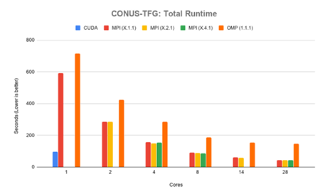
4.1 CONUS-TFG: Total runtime in seconds. . . . . . . . . . . . . . . . . . . . . . . . .
4.2 CONUS-TFG: Runtime for NL Function Eval in seconds . . . . . . . . . . .
4.3 CONUS-TFG: Runtime for MG Semi in seconds . . . . . . . . . . . . . . . . . .
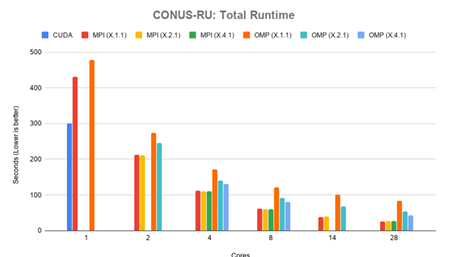
4.4 CONUS-RU:Total runtime in seconds. . . . . . . . . . . . . . . . . . . . . . . . . .
4.5 CONUS-RU:Runtime for NL Function Eval in seconds . . . . . . . . . . . .
4.6 CONUS-RU:Runtime for MG Semi in seconds. . . . . . . . . . . . . . . . . . . .
4.7 ClayL:Total run time in seconds. . . . . . . . . . . . . . . . . . . . . . . . . . . . . . .
4.8 ClayL: Runtime for NL Function Eval in seconds . . . . . . . . . . . . . . . . .
4.9 ClayL: Runtime for MG Semi in seconds . . . . . . . . . . . . . . . . . . . . . . . .
5.1 Kernel stages with scheduling expressed in the STELLADSL. . . . . . . .
5.2 2D Blur Algorithm Pseudo code . . . . . . . . . . . . . . . . . . . . . . . . . . . . . . .
5.3 2DBlur Algorithmin Tiramisu . . . . . . . . . . . . . . . . . . . . . . . . . . . . . . .
5.4 4th Orderx-Flux Smoothing in STELLA. . . . . . . . . . . . . . . . . . . . . . . .
LIST OF ABBREVIATIONS
HPC
High Performance Computing
DSL
Domain Speci c Language
eDSL
Embedded Domain Speci c Language
CONUS
Continental United States
UVA
Uni ed Virtual Addressing
MPI
Message Passing Interface
GPU
Graphics Processing Unit
GPGPU
General Purpose Graphics Processing Unit
CHAPTER 1
INTRODUCTION
Legacy scienti c applications represent signi cant investments by universities, engineers, and researchers and contain valuable implementations of key scienti c computations. Such applications are used in a wide range of research elds including medical imaging [25], industrial manufacturing, climate modeling [24, 2], geology, hydrology, and others. Computational scientists continuously update these applications to improve the underlying mathematical models and port the code to the latest hardware. However, years of updates to mathematical formulations, porting to new hardware, and optimizing for new hardware capabilities complicate code bases, making them difficult to maintain and extend. Computational scientists need abstractions that separate key computations from hardware speci c implementation details, isolating the code complexity that comes with these issues.
There is a signi cant need for abstractions to provide the three Ps: Productivity, Portability, and Performance. Productivity is paramount, representing how well and easily a scienti c programmer can implement new simulations of scientific models; productivity directly correlates to scienti c impact. As new hardware emerges, implementation details in the code change. Abstractions must provide a layer between computations and the necessary underlying implementations to allow for architecture portability. This additionally contributes to scientific impact, as the longer computations take the less research can be performed in a given period of
time. As new architectures develop, they o er potential increases in computational throughput. Portability is the ability to run an application across multiple architectures. Porting existing code to new architecture is time consuming and expensive.
Abstractions allow for core computations to be separated from architecture specific implementation details. This allows for portability without the need to rewrite computations. Therefore abstractions that manage this process are highly desirable. Performance is a measurement of how long an application takes to solve a particular problem. Abstractions must be exible enough to allow for architecture specific optimizations. Di erent architectures have di erent implementation requirements to achieve good performance, and this must be realized without significant changes to the computations themselves.
This thesis presents a series of abstractions designed to improve scienti c programmer productivity by separating architecture specific code details from the primary computations. This separation provides a way to implement architecture specific optimizations without obfuscating code, and without the need to rewrite computations. The abstractions are generally applicable to many applications, and are demonstrated with ParFlow, a hydrologic modeling platform.
ParFlow is representative of a class of scienti c applications that solve partial differential equations. These applications all include boundary conditions, and many frameworks exist to handle them including CHOMBO [32, 28, 3], AMReX [48], ForestClaw [10], and ClawPack [24]. Boundary conditions are critical to solving partial differential equations. There is a clear need for abstractions that maintain productivity while enabling architecture portability and improving performance.
1.1 Problem Statement
Code complexity in legacy scientific applications caused by years of updates prevents computational scientists from implementing new computations and mathematical models, degrades application performance, and impedes architecture portability.
1.2 Case Study: ParFlow
ParFlow is a hydrologic modelling application that simulates surface and subsurface water ow through porous materials. It is a highly modular platform, allowing for a wide range of simulations and research to be performed. The domains that are simulated in ParFlow may be based on real world geometry, such as the Continental United States, or may be synthetic. ParFlow rst solves a steady state equation across the domain, then performs calculations to handle boundary conditions. The original developers of ParFlow saw the need for scalability, but presently this is limited to MPI only. Part of this thesis is to provide portable on-node, shared memory parallelism for multicore systems and accelerators.
Productivity. Over the course of its lifetime, the codebase in ParFlow has become highly complex. As a result, computational scientists have had difficulties in extending mathematical models. An instance of this is the addition of new bound ary conditions. Computational scientists have been unable to add new boundary conditions to ParFlow models for 15 years due to code complexity issues. Boundary conditions are crucial to the development of new watershed models, and this represents a signi cant loss of scienti c impact. This demonstrates the immediate need for productive abstractions.
Portability. Di erent problem models have di erent computational resource requirements. A small problem may have very low computational requirements and could be run on something like a laptop. Larger and more complex problems may have significantly greater computational requirements, and necessitate the use of a
supercomputer. ParFlow must be able to run across these di erent compute resources, from a laptop to a leading class supercomputer. Available hardware changes between compute resources and over time, and di erent hardware architectures have specific implementation requirements. Rewriting code to t these architecture speci c requirements is prohibitively expensive. This is compounded over time as new hardware architectures are developed, requiring rewrites for each one. ParFlow has a clear need for architecture portable abstractions that do not require the rewriting of key computations.
Performance. Applications that solve complex problems take time to execute. The more complex the problem becomes, the longer it takes for the application to solve. Computational resources consume significant amounts of electricity, and the longer an application must run the most electricity is used. The worlds leading supercomputer, Summit at Oak Ridge National Laboratory, consumes as much as 10 megawatts of energy [1]; as much as an entire city. This is both nancially and environmentally costly. As computational scientists extend their models in ParFlow, the computational resources required increase. Performance must be improved to meet these new requirements, reducing nancial and environmental costs, and improving scientific impact.
1.3 Contributions
This thesis contributes a proposed design of abstractions for boundary condition computations. The abstractions are generalizable to other scienti c applications. ParFlow is used to demonstrate the e ectiveness of the abstractions. The abstractions have improved computational scientist productivity in ParFlow, and enable
architecture portability.
An experimental OpenMP version of ParFlow was implemented using the abstractions. This demonstrates a realization of architecture portability in the abstractions, without signi cant rewriting of computations. A performance study was conducted, comparing on-node shared memory performance of MPI, OpenMP, and CUDA versions of ParFlow. This study examines performance in different congurations of a real scientific application, and explores the complexities involved.
1.4 Organization
This work is organized into several chapters and sections. Chapter 2 provides back ground on ParFlow, boundary conditions, and architecture portability. Chapter 3 covers the abstractions developed, their design, and the steps necessary to perform boundary condition computations. Chapter 4 provides a performance study, comparing the different experimental versions of ParFlow. Chapter 5 contains a review of related work and other DSL abstractions. Chapter 6 concludes and summarizes this work.
CHAPTER 2
BACKGROUND
The abstractions developed in this work are applicable to a wide range of scientific applications. We demonstrate their e ectiveness using the ParFlow application. This section provides a brief overview of ParFlow, with a focus on boundary conditions and domain decomposition. Challenges in architecture portability with respect to
OpenMP and CUDA are also presented.
2.1 ParFlow
ParFlow is a hydrologic and geoscience application that integrates multiple water shed models [30, 5, 27, 23], and is part of the HydroFrame [38] project. The HydroFrame project aims to simulate ground water ow for the Continental United States (CONUS) and increase accessibility of integrated hydrologic simulations to a larger community of hydrologists and educators. ParFlow models the ow of water through porous material using Richards equation integrated with overland ow using Mannings equation. ParFlow utilizes a coupled model for simulating surface and subsurface overland ows. It is a well-established research tool within the hydrology community, with on-going work to improve its mathematical models for new simulations.
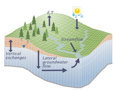
ParFlow simulates the ow of water through a domain. The domain may represent a real area and include historical atmospheric data, a real area with predicted or hypothetical atmospheric data, or represent a synthetic area that represents a physical area. Once con gured, ParFlow discretizes the problem domain into a collection of
grids. These grids are split across the X, Y, and Z axes. The Z axis represents depth of the domain, while X and Y represent the horizontal regions of the domain. Each grid is further discretized into subgrids, and each subgrid discretized into cells. Figure 2.1 is an illustration of a domain that has been divided into grids, subgrids, and cells. Cells represent the data points in the model, and are the operands to the computations. This particular discretization is called an orthogonal grid, where cells are equally distributed across the domain. Par Flow uses Richards equation to solve for variably saturated groundwater ow (2.1).

(2.1)
Richards equation is well known [40], and describes the relationship between subsurface pressure heads, hydraulic conductivity, permeability of soil, saturation, and exchange rates with the surface. The discretized form of this equation forms the steady state stencil equation. Computations are performed using stencil patterns. The use of stencil patterns in scientific computing is common [18, 13, 37]. A stencil pattern involves reading a cell and some set of neighbors to calculate a cells value in the next iteration. Grids, and their associated subgrids and cells, may exist on the edge of the model domain. Cells that reside in these locations are part of the boundary. Boundary cells lack at least one neighbor needed to perform the stencil computation. A boundary condition is the computations to be performed in place of the stencil, also called the steady state equation. A boundary cell will have a condition for each face along the boundary.
2.1.1 Boundary Conditions and CONUS
A cell in the very corner of a domain may have an overland ow boundary on its top face, and constant ux boundary conditions on its horizontal faces. Boundary cells represent areas with different physics and computational requirements. Examples of boundary conditions include overland ow on the surface, such as a river, atmos phericuxes such as rainfall or snow, or constant ux values such as a river head. The cells in these regions account for water ow into or out of the domain, and are essential to scientific models. Boundary conditions can exist in surface regions, as well as subsurface regions.
ParFlow uses a free surface overland ow boundary condition to swap between solving subsurface and overland ow equations when water is ponded on the land surface of the model [27]. This is a coupled model that handles boundary condition cells on the surface that have water in ow or out ow occurring. As an example, consider a boundary condition cell on the surface of a model with rainfall. There is no immediate neighbor on the top of this cell, but the ow of rain into this cell must be included in computations. This coupled surface-subsurface model accounts for these overland boundary conditions. These are Neumann type boundary conditions, but can be switched to Dirichlet if necessary.
The HydroFrame project aims to create a more comprehensive model of the continental United States. CONUS 1.0 is a model that simulates subsurface and groundwater ows across a large section of the continental United States, but as can be seen in Figure 2.2 only a rectangular inset of the continent is modelled. CONUS 2.0 is an update to this model and will include more complex coastal regions and geological areas. Boundary condition development is critical to this new model in order to provide the necessary computations for these new regions.
Boundary conditions are computationally intensive, and the inclusion of large, complex coastal regions in CONUS 2.0 creates a need for improved performance. Additionally highly complex implementation details in the codebase prevent the development of new boundary conditions, posing a direct barrier to the development
of CONUS 2.0. This highlights the immediate need for intuitive abstractions to improve for computational scientists to use in developing new boundary conditions. These abstractions must also provide architecture portability, and allow for improved
![Figure 2.2: The CONUS 1.0 Domain [29]](https://bulgariantimes.org/wp-content/uploads/2024/03/figure-2.2.png)
2.2 Domain Specific Languages
ADomainSpeci c Language is a method of abstracting common idioms in a codebase. This is most often seen in terms of expressing complex or common looping patterns, but is also used for memory allocation and data structure manipulation. DSLs provide an interface for developers that reduces code complexity, improving productivity. Additionally, domain speci c languages can help to enable architecture portability, as the back-end structure can be modi ed to accommodate new architectures without needing to significantly change the developer-facing interface. Similarly, domain specific languages help improve application performance by allowing performance
optimizations to be done on the back-end. DSLs are often written in the form of a
library, but can also be embedded within a program, known as an eDSL (embedded DSL). In this context embedded means speci c to the application, with no external library dependencies or additional compiler required. Other DSL e orts in atmospheric and hydrologic science are discussed in Related Work, Chapter 5.
2.2.1 Existing ParFlow eDSL
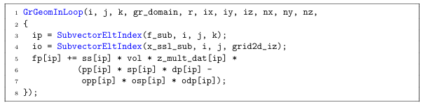
ParFlow contains an existing eDSL, primarily used for navigation of the model domain when performing computations. The eDSL abstractions encapsulate steady state computations, but leave boundary condition implementations exposed. As a result, complex control ow must be manually con gured and managed by scienti c programmers, hampering productivity and preventing architecture portability to GPU accelerators.An example of the existing eDSL for steady state computations can be seen in Figure 2.3. This example, GrGeomInLoop, is used to navigate through the interior cells of the 3D model domain and perform computations accordingly. Iteration starts at ix, iy, iz up through nx, ny, nz. The SubvectorEltIndex abstraction handlesmapping the iterators to memory locations for scientific programmers, providing ausable accessor index for reading and writing into data.
2.3 Architecture Portability
Legacy scienti c applications have long lifespans, and over the course of those lifetimes hardware changes dramatically. ParFlow was originally developed for single core processors and modern processors are much di erent. Abstractions provide a single front-end view of computations, and allows complex architecture-speci c code to be hidden. This section describes two target paradigms: multi-threaded execution through the OpenMP framework, and many-core GPU execution through CUDA.
2.3.1 OpenMP
OpenMP is a community driven API for directive based multi-threaded, shared memory programming [35]. Compile-time directives are inserted by the programmer to indicate how work should be distributed and where threads must synchronize, or when work can or cannot be done in parallel. Additional directives can be specified to indicate whether a variable can be shared between all threads, or must be private to each thread.
Aset of commonly used directives, also called pragmas, include omp parallel, omp for, omp master, and omp single. The omp parallel directive declares that a region of code should be performed in parallel, with optional clauses to declare speci c variables shared or private. The omp for directive speci es that a loop should have its iteration
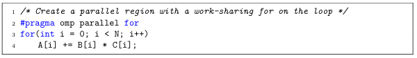
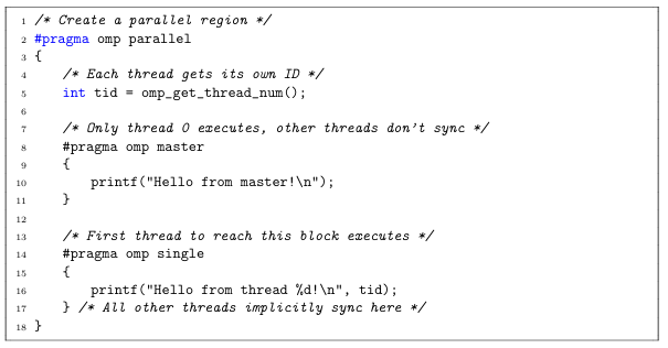
space divided among threads when inside of an omp parallel region. The omp parallel and omp for directives can be combined into omp parallel for when only a loop needs to be performed in parallel. Figure 2.4 shows an example of this, where a parallel region is created and the for loop distributed among threads. The omp master and omp single directives are used within parallel regions, and indicate that only a single thread should execute a given block of code. The master directive means only the thread with id 0 will execute, and all other threads can continue without synchronization. The single directive means the rst thread to encounter the directive will execute, but all threads must synchronize at the end of the directive. Figure 2.5 illustrates this by creating a parallel region, in which only the master thread will print the rst statement and only a single thread will print the
second. OpenMP provides more directives, all with optional clauses to provide different functionality including memory management, scheduling, and synchronization. Exposed OpenMP directives introduce additional layers of complexity in managing parallelism and synchronization. As a result the directives must be abstracted away from scientific programmers in order to reduce code complexity and maintain productivity.
2.3.2 CUDA
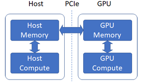
GPU accelerators o er enormous parallelism, but existing code must be carefully adapted to make use of them. A GPU accelerator consists of thousands of threads that are grouped together in warps, with 32 threads per warp. Execution on a GPU accelerator is performed through the use of Kernels. A kernel is a function compiled by the GPU compiler for execution on the accelerator. Invoking a kernel requires the transfer of data in host (CPU) memory to device (GPU) memory, seen in Figure 2.6.
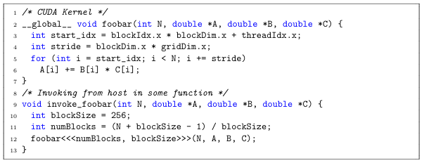
This transfer can be done explicitly, or though the use of a memory manager such as CUDA Uni ed Virtual Addressing [42] (UVA). UVA allows the CUDA runtime to map host and device memory into a single address space, and automatically transfer memory as necessary. This introduces costly overhead, but greatly simplifies development. An example of a kernel performing a streaming computation can be seen in Figure 2.7. This example assumes the transfer of data from host to device is being done through UVA, or has otherwise already occurred. Memory transfers occur through the PCIe bus, which has signi cant overhead costs. This transfer can become prohibitively expensive and must be managed carefully to achieve good performance on a GPU.
The layout of threads to be used in computation on the GPU must be speci ed. GPUaccelerators allow for threads to be con guring in di erent dimensions, aecting memory access patterns. This con guration of threads can be seen in Figure 2.7 when
the host invokes the kernel, lines 10 through 12. When the kernel is invoked, each thread in the warp calculates a starting index based on the con gured thread layout, seen on line 3. A striding factor is calculated similarly on line 4. This makes the loop parallel, with each thread accessing data in independent indices than all other threads.
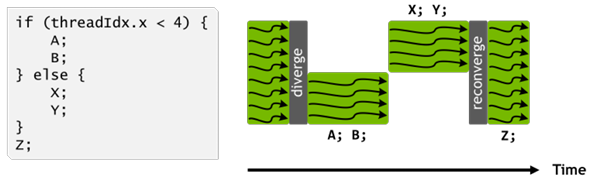
When a kernel is invoked, execution on the GPU begins. All threads in a warp operate in lockstep, only di ering in the data they operate on. This produces an issue known as thread divergence, in which one thread encounters a conditional branch that others do not. When this occurs, all other threads that do not enter this branch must perform a no-op instruction [20], and do nothing until the branch is complete. This then repeats for the threads that entered the branch in turn. Figure 2.8 illustrates this, where a group of threads encounters a conditional branch. Half of the threads will enter one branch, executing statements A and B, while the other half remains idle and performs a no-op instruction. Once the rst half has nished executing, the second half will execute statements X and Y, with the rst half similarly remaining idle. All threads then synchronize and can continue in lockstep, executing statement Z. Thread divergence results in loss of performance and wastes compute resources, and is an area of active research [43, 19].
The implementation details of GPU accelerators become complicated quickly, increasing code complexity through memory management, synchronization, kernel invocations, and control ow. These details must be abstracted from scienti c programmers to ensure productivity, while still providing performance benefits.
CHAPTER 3
BOUNDARY CONDITION ABSTRACTIONS
The proposed boundary condition abstractions are designed to improve productivity, provide portability, and allow architecture-speci c optimizations to improve performance. The abstractions separate architecture-speci c implementation details from primary computations. This reduces code complexity without requiring computational scientists to rewrite or reformulate computations, improving productivity. Several architecture-speci c backends can be implemented without changing forward facing code, providing portability. Di erent backend implementations can then have architecture-specific optimizations applied, improving performance. Boundary condition computations are used in several ways, and ensuring long-term productivity improvements requires the abstractions provide full coverage. Full coverage means that all use cases of boundary condition computations are fully encapsulated by the abstractions. This chapter will cover the design approach for the new abstractions, the abstractions themselves, and the architecture portable backends for OpenMP.
3.1 Design and Approach
Computational scientists actively participated in the design of the abstractions. Their participation ensured that productivity goals were met, resulting in a clear and intuitive design. We implemented backends iteratively during the development of the frontend abstractions to verify minimal overhead, and ensure portability goals were met. The result is a set of powerful abstractions that computational scientists are comfortable working with, and that computer scientists are able to use to produce effecient code. Boundary conditions are interacted with in several sections of the application. During the con guration stage the different types of boundary conditions are set and the domain is de ned. This involves setting the source of boundary condition values (Section 3.1.1), and setting appropriate data for each time step in the model (Section 3.1.2). The values are then used at each time step to perform boundary condition computations (Section 3.1.3). The following sections detail this process.
3.1.1 Setting the source of Boundary Condition Values
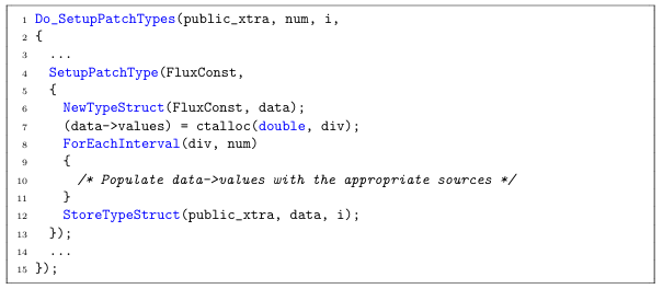
Boundary conditions must be con gured before the execution of the model begins. The first step in this con guration is to de ne the sources for boundary condition values. Abstractions were provided to facilitate this step in an intuitive way that is self-describing. These abstractions manage the allocation, storage, control ow, and enumeration of the necessary data for different boundary condition types. Figure 3.1 is an example of setting up source values for a FluxConst boundary condition type. Do Setup Patch Types (line 1) accepts a list of boundary condition types and the details of how their source values are congured. Each boundary condition
type will have a Setup PatchType (line 4) entry inside of the Do SetupPatchTypes interface. SetupPatchType contains the con guration details for a speci ed boundary condition type and provides an interface for allocating memory, populating initial values, and storing the data. NewTypeStruct (line 6) allocates a data structure of the appropriate type used to store data source information. For EachInterval (line 9) iterates over all time steps for the model being executed, and contains the implementation details to populate source values. StoreTypeStruct (line 13) stores the data structure for later retrieval.
3.1.2 Setting Data For Each Time Step
Once the source locations for each boundary conditions data has been set, data for each time step in the model is prepared. Figure 3.2 shows an example of setting initial timestep values for a FluxConst boundary condition. ForEachInterval (line 1) iterates over all timesteps in the model being executed. Do SetupPatchIntervals (line 2) accepts a list of boundary condition types and the details of how their values are con gured. Each boundary condition type will have a SetupPatchInterval (line 5) entry inside of the Do SetupPatchIntervals interface. Setup PatchInterval contains the con guration details for a speci ed boundary condition type and provides an interface for allocating memory, retrieving source values, populating initial time step values, and storing data.
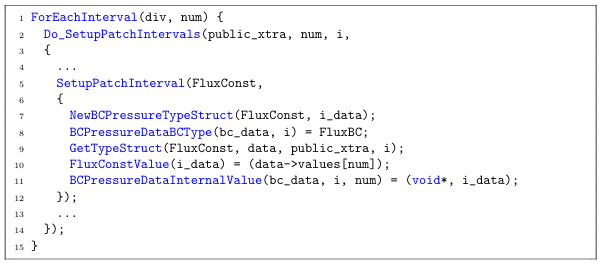
New BC Pressure Type Struct (line 7) allocates a new data structure for the specified boundary condition. BCPressureDataBCType (line 8) assigns the categorical type of boundary condition, used to determine what computations to perform using the data. For example the FluxConst and FluxVolumetric types have different details for con guring initial values, but use the same mathematical computations and are of the FluxBC category. GetTypeStruct (line 9) retrieves the source values that were previously con gured. FluxConstValue (line 10) is an acccessor into the data structure, used in this example to store the particular value for a given timestep. Each boundary condition type has its own set of accessors accordingly. BC Pressure DataInternal Value (line 11) stores the timestep data structure for retrieval and use in computations.
3.1.3 Performing Boundary Condition Computations
Boundary condition computations are used in di erent ways throughout the ParFlow codebase. It is necessary to be able to apply different computations for different types of boundary conditions. There are instances in which all boundary condition types perform the same set of computations, such as to adjust coe cients when dealing with symmetric Jacobian matrices.
Different computational use cases have been identi ed and a set of consistent abstractions developed.
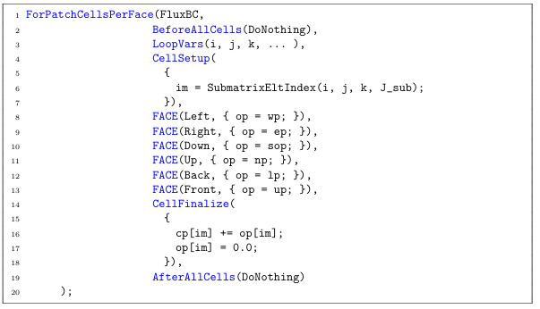
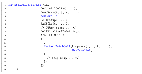
Boundary condition computations can be decomposed into ve primary sections. Asimple example of a Flux boundary condition computation, pulled from the Richard sJacobianEval function in ParFlow, can be seen in Figure 3.3. The rst section is a block that must occur before looping over the cells of the boundary condition patch, named BeforeAllCells (line 2). This allows for a block of code to be executed unconditionally before boundary condition computations are performed across cells. An example of this may be some uniform scalar setup from a function call, so that the function call is not repeated for every cell iteration. Another example may be a nested boundary condition loop that counts some number of values across all cells for data allocation.
The next section is CellSetup (line 4). This is a region that is used for setting up values to be used in the computation on the current cell, such as preparing accessor indices or calculating a scalar used in computations. Previously control ow was managed manually by computational scientists to determine which directions were valid for the current boundary condition cell, increasing code complexity. This is replaced with the next section, containing a set of FACE (lines 8- 13) entries. Each FACE speci es the direction it represents, and contains the appropriate computations to be executed. A boundary condition cell may have multiple valid directions, but only one is valid at a given iteration. For example a cell on the corner of the domain may have two valid faces, but the appropriate face computations will happen in separate iterations.
The final two sections are CellFinalize (line 14) and AfterAllCells (line 19). CellFinalize is the counterpart to CellSetup, and is where the result of computations performed in the FACE section are utilized. AfterAllCells is similarly the counterpart to BeforeAllCells, and will unconditionally execute after every cell in the boundary condition has been iterated over. The DoNothing keyword (lines 2, 19) is provided for sections that are unnecessary for the computations being executed
Di erent regions of code in ParFlow loop over boundary condition cells at different points. Control ow for branching on boundary condition types may be hoisted far away from the loop itself, such as outside of the function. Computations may also apply to all boundary condition types, such as for handling contributions for a symmetric Jacobian matrix. For these cases, the ALL keyword (Figure 3.4 line 1) can be used in place of a speci c boundary condition type, causing the loop to execute unconditionally. There may also be no special computations for each face
direction. In this case, the ForEachPatchCell abstraction is provided (Figure 3.4, lines 4 and 28). Finally, the iteration space may need to reach into ghost cells. A ghost cell is used to exchange data between MPI processes. The For Patch CellsPer Face And Ghost abstraction is provided to facilitate this, and works identically to the
For Patch Cells Per Face abstraction. The use of these abstractions removes the need for computational scientists to manage control ow manually, and separates implementation specific details from the computations. This is done in a way that does not require computations to be rewritten, and allowing computational scientists to continue writing code in a way they are comfortable with, maintaining and improving productivity. These
abstractions are expressive and exible, and can be nested within each other. An example of this can be seen in Figure 3.4, where the patch is rst iterated over to count the number of cells for data allocation, iterated over a second time to calculate a necessary scalar, and then iterated over a third time to compute and store data.
These abstractions separate the concerns of the mathematical computations used in boundary conditions from the speci c implementation details. Code complexity is reduced, with cleanly separated blocks that clearly de ne what is being done inside of them. Control ow is no longer dealt with directly by computational scientists. This provides architecture portability, as the implementation and computations are no longer tightly coupled.
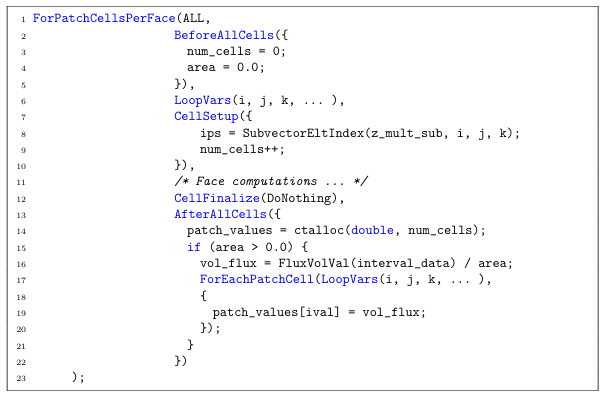
The reduced code complexity helps to highlight potential loop fusions. An example of this can be seen in Figure 3.4. This gure shows how the original code ordered the sequences of loops. A full iteration over all cells in the boundary condition is performed to count cells for data allocation. A second iteration over all cells in the boundary condition performs an accumulation into a variable. Finally, if that variable
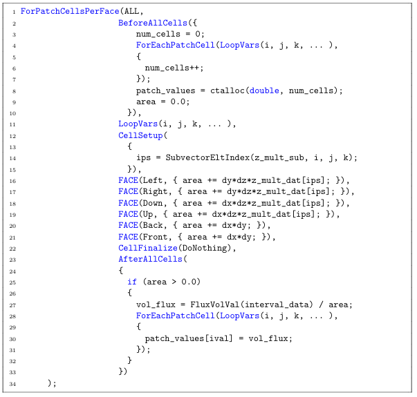
is not zero,a third iteration over all cells in the boundary condition populates values for use in later computations. In the new abstraction it becomes clear that this first iteration is unnecessary. The number of cells is not used until after the are a variable has been calculated,and so the first loop can be merged in to the second. This can be seen in Figure 3.5, reducing total iterations from 3Nto2N.
loop fusion
3.2 Backend Development
The new boundary condition abstractions have enabled the development of experimental ParFlow builds for OpenMP. OpenMP was chosen for on-node memory sharing performance, providing a wide range of compile-time hints and instructions for improved threading performance. The complex control ow in the original boundary condition implementations posed barriers to parallelism with OpenMP directives and thread divergence on GPU accelerators. The proposed abstractions separate computations from architecture speci c details. This permits implementation details to be hidden and prevent increased code complexity. Beyond boundary condition loops, ParFlow contains several existing looping abstractions that were modified for
portability with minimal forward-facing changes.
3.2.1 Data ow and Pro ling Analysis
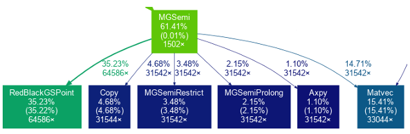
Before implementing new backends, pro ling of ParFlow was performed to identify time-dominating functions and their subroutines. Due to the highly con gurable nature of ParFlow, this pro ling focused on the test cases discussed further in chapter 4. Initial pro ling was performed using the GNU gprof [17] utility. Figure 3.6 is a subsection of the call graph of one of the test cases, generated by gprof and run through the gprof2dot [15] utility for visualization. Each node represents a function and consists of the name of the function, percentages of total runtime, and number of times the function was called. The rst number is the percent of cumulative time spent in the function or its subroutines against the total runtime of the application. The second number, listed in parenthesis, is the percentage of time spent directly within the function. The third number is total number of calls to the function. Once time dominating functions were identi ed, data ow analysis was performed. This was done in order to identify serial optimizations that can be applied to all versions of ParFlow, as well as to identify necessary synchronization barriers in OpenMP. This was performed and recorded manually as a set of Macro Data ow Graphs, which represent data dependencies, computational statements, and data points as nodes within a directed acyclic graph. Macro Data ow Graphs and their use for automatic, compile-time transformations and optimizations is an on going area of research [14].
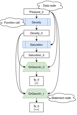
Graphs are read from left to right, top to bottom. Nodes indicate their meaning by their shape, and directed edges indicate data dependencies and data ow. Nodes that are shaded gray are immutable and cannot be transformed. Data nodes contain the name of the variable they represent, with a subscript to indicate when they have been assigned to in a single-static assignment view. In this context, commutative operations such as addition (+ =) or subtraction ( =) into a data node is not considered a new assignment, as they can be rearranged with the same mathematical result. The full list of node types are:
.Rectangle- Data node, containing the variable name it corresponds to and a subscript to indicate its assignment count.
.Trapezoid- Statement node. These are seen as inverted triangles in other work, but due to software limitations a trapezoid was used in these graphs. These nodes represent loop patterns in this context.
Rectangle with side-bars- Function call node.
Directed edge- Data dependency and data ow.
A directed edge going into a node indicates a data dependency. A directed edge coming out of a node and into a data node indicates a new assignment to that data. A subsection of the data ow graph for the function NL Function Eval can be seen in Figure 3.7. Starting from the top, a call to the Density function is made reading data from the Pressure 0 node. This emits the data node Density 0. A call to Saturation is made, similarly reading data from Pressure 0 and Density 0, and emitting Saturation 0. Two loops occur sequentially, reading data as indicated by the connected edges, and emitting nodes. These graphs were prepared through analysis of the original codebase, and were used to identify areas that required parallelism barriers such as MPI communication. Potential loop transformations such as loop fusion [8, 7] or loop tiling [39] were also identified using these graphs.
Figure 3.7 shows that there are no direct loop-carry dependencies between the loops GrGeomIn 0 and GrGeomIn 1. A loop-carry dependency is where one loop
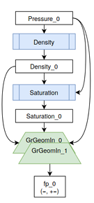
modifies data that is used in a subsequent loop. This indicates there is a potential for loop fusion. Figure 3.8 is an example of the data ow graph after performing a loop fusion. The full data ow graph for NL Function Eval can be found in the appendix, showing it is possible to fuse 4 loops. This can be accomplished by reordering loops in the function and performing temporary storage transformations. These transformations were not applied in order to provide a baseline in the performance study, detailed in Chapter 4.
3.2.2 OpenMP
The design of the new boundary condition abstractions enabled rapid development of an OpenMP implementation. An additional parameter was added to abstractions, indicating one of several sets of OpenMP directives to be used across the interior looping structure. An example of this can be seen in Figure 3.9, where lines 4 and 13 contain an additional NewParallel clause. The NewParallel clause creates a new OpenMP parallel region and distributes the loop computation across multiple threads. Additional keywords exist to indicate that the loop is already in parallel region, make certain variables thread-private, perform reductions, or to skip implicit synchronizations with the no wait clause. This provides clear indications of what kind of parallelism is being applied without increasing code complexity. This parame terization was applied similarly to other looping patterns, such as for steady state equations.
Time dominating functions were analyzed and several challenges to the implementation of OpenMP identi ed. These challenges include but are not limited to synchronization, data races, mixing MPI barriers with OpenMP, iteration calculations, and managing large parallel regions across multiple function calls. Initial development was performed by analyzing each looping structure within a function to determine possible parallelism. Looping structures that were not immediately parallel had further analysis performed to identify methods that may provide parallelism. Examples of these include storage duplication and managing scatter-gather patterns. Once parallelizable, each looping structure was isolated into individual parallel regions. This means that at the beginning of the iteration space, a thread group would be requested. The body of the iteration space would be divided amongst threads and performed in parallel. Temporary scalars can be made thread-private with optional directives. At the end of the looping structure, all threads synchronize, and the program returns to serial execution.
Next, explicit parallel regions would be declared at an appropriate place in the beginning of the function. Parallel loops would be incrementally incorporated into the region to help manage and debug race conditions and synchronization issues. The use of a parallel region reduces the overhead associated with requesting thread groups and unnecessary synchronizations. Because of the abstractions, typically only a single keyword needed to be changed when moving a loop from an isolated parallel region to an incorporated one, or to add and remove barriers. Once a subroutine was able to be run in parallel from start to end, the process was repeated in its parent function. Parallel regions were explicitly declared, and isolated parallel loops would be incorporated. This followed by incorporating the subroutines into the parallel region, with each thread entering it and maintaining the bene ts of Open MP directives. Signi cant data analysis was required for this to identify race conditions and eliminate unnecessary synchronization points. As ParFlow was originally developed to be an MPI-Only application, there are frequent calls to perform updates between MPI processes. MPI calls in a hybrid MPI-OpenMP implementation require explicit synchronizations so that data being exchanged between MPI processes is not modi ed by other threads. This is a common challenge when moving an application from MPI-only to a hybrid MPI-OpenMP implementation [36, 41]. The Scalasca performance tookit [16] was utilized to help identify regions of code resulting in synchronization issues, as well as general multi threaded pro ling.
3.2.3 Limitations
The use of keywords in development of OpenMP, such as NewParallel, poses limitations in regards to productivity. In order to safely add new mathematical formulations, computational scientists now need to understand parallelism concepts such as synchronization, race conditions, and more. A possible solution is to perform static analysis to determine where no synchronization is needed, or where a variable needs to be declared thread private. Transformations on the backend could then automatically be applied, such as removing synchronization barriers in OpenMP or CUDA. Addressing these limitations through static analysis is beyond the scope of this work.
CHAPTER 4
PERFORMANCE STUDY
This section details a performance study of experimental builds of ParFlow. A set of test cases were chosen with computational scientists. This performance study is done to examine the shared memory performance of MPI, OpenMP, and CUDA implementations of ParFlow. The OpenMP and CUDA versions are experimental. This study found that OpenMP outperforms or is competitive with MPI under certain con gurations, and that CUDA outperforms MPI in some con gurations.
4.1 Benchmark Suite
ParFlow is highly con gurable, and di erent con gurations result in large variations in performance characteristics. A model can be con gured with di erent settings, including maximum number of solver iterations, tolerance values, number of time steps, domain sizes, and solver types. This creates an exponential number of combination, not all of which may make sense. Computational scientists were consulted and a set of useful domains were chosen as test cases. These test cases were used to examine the feasibility of the experimental versions of Par Flow ; analyzing performance in di erent domains and key sections of ParFlow. Performance was analyzed in the context of a single compute node to measure shared memory and GPU performance compared
to the baseline MPI implementation. Selected test cases include: CONUS Terrain Following Grid (CONUS-TFG), CONUS Runo (CONUS-RU), and ClayL. CONUS-TFGis a subsection of the CONUS 1.0 model in Colorado, with multiple Z layers and real slope geometry. TFG stands for Terrain Following Grid. When using a terrain following grid, the orthogonal grid discussed in 2.1 is transformed to conform to the problem domain topography on both the surface and subsurface layers to exclude inactive areas [31]. This is bene cial when overland ow closely follow the topography.
CONUS-RU is a subsection of the CONUS 1.0 model in southern Colorado, with a single Z layer and real slope geometry. CONUS-RU is known as a parking lot model where permeability is set to near 0, preventing water from entering the subsurface of the domain. This pools water across the domain, and identi es where rivers, streams, and sinks exist. Parking lot models are used frequently when developing simulations for new domains.
ClayL is a synthetic domain consisting of homogeneous soil and a large Z depth, with no complex terrain. ClayL is included in this study as it is used for acceptance testing of supercomputers in Europe.
4.2 Experimental Setup
Testing was performed on the R2 cluster at Boise State University [44], running from 1 to 28 cores on a single node. A node on the R2 cluster is con gured with two Intel Xeon E5-2680 v4 14 core CPUs running at 2.4ghz, with 192GB of memory split into two NUMA nodes (96GB per CPU socket). CUDA performance was measured on a GPU node with two Intel Xeon E5-2680 v4 14 core CPUs running at 2.4ghz, with 256GB of memory split into two NUMA nodes, and an Nvidia Tesla P100 GPU. The links to the speci c git commits used for each version can be found in Appendix A. ParFlow was compiled with GCC 7.2.0 using the O3 ag, and NVCC 10.0.130 was used to compile the CUDA version. MPICH 3.2.1 was used for MPI. Results compare ParFlow running with MPI, the experimental OpenMP implementation, and an experimental CUDA version. The experimental CUDA version was provided by the Juelich Research Center in Germany. MPI communication is currently not supported in the experimental CUDA version, and is only run on one CPU core with one GPU accelerator. The CUDA version of ParFlow does not use the abstractions presented, instead being hard coded to run on GPU accelerators. However, the abstractions are able to support a uni ed CUDA implementation.
4.3 Results
This section presents the results of the performance study. It is important to note that ParFlow utilizes KINSOL, a nonlinear solver for algebraic systems that is part of the SUNDIALS library [21]. KINSOL is developed by Lawrence Livermore National Laboratory, and analysis for implementing OpenMP or CUDA in it is beyond the scope of this work. Analysis shows that the CUDA and OpenMP versions take a signi cant performance penalty due to the KINSOL library being single threaded. MPIdoesnotseethis penalty as every MPI process has its own copy of the application, allowing KINSOL to be run in parallel. MPI does not see this penalty as every MPI process has its own copy of the application, and so KINSOL can be run in parallel.
The results for two time dominating functions, NL Function Eval and MGSemi, are included to exclude the overhead from KINSOL in OpenMP and CUDA. This is done
Table 4.1

to examine the performance of OpenMP, CUDA, and MPI in parallel regions of code. Con gurations for each test case are detailed at the beginning of each subsection. Total runtime, and runtimes spent in NL Function Eval and MGSemi are examined. Full timing results for all test cases for 1 to 28 cores can be found in Appendix B. A comparison between ParFlow without the abstractions and with the abstractions was run for each test case on 28 cores, seen in Table 4.1. The abstractions involve changes to the codebase. This can result in di erent compiler optimizations and execution orderings, resulting in time variations. System interrupts, le IO operations, and general system noise contribute further variations in timings. These results show that the abstractions do not have significant negative impact on runtime using 28 cores.
4.3.1 CONUS-TFG
The CONUS-TFG test was run in several MPI con gurations. These are denoted as (X.1.1), (X.2.1), and (X.4.1) where X is a varying number of cores. ParFlow decomposes a domain as the product of the provided con guration. For example a
decomposition of 7.4.1 will split the domain along the X axis 7 ways and the Y axis 4 ways, and distribute data to 28 cores. Domain decomposition has impact on memory layouts and domain traversal, and is under exploration. The OpenMP version was run on one MPI process, with a varying number of threads. Full timing results for 1
to 28 cores can be found in Appendix B Table B.1. Figure 4.1 shows the total runtime for the CONUS-TFG test case in seconds. CUDA performed faster than MPI in all con gurations until more than 8 cores are in use. The CUDA version solved the problem domain in 95.14 seconds. The MPI version performed equally between each of its con gurations, with the fastest time of 41.87 seconds in the 14.2.1 con guration for a total of 28 cores. OpenMP was consistently slower than MPI in this test case, with 28 cores solving the problem domain in 146.08 seconds.
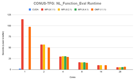
Figure 4.2 shows timing results for NL Function Eval in seconds. The CUDA version performed faster than all MPI con gurations up to 28 cores, spending 2.14 seconds in this function. The MPI version performed equally between all con gurations. The fastest time for MPI was in the 14.2.1 con guration, spending 5.30 seconds in the function. OpenMP performed faster than all MPI con gurations until more than 8 cores are in use, at which point it became competitive. OpenMP spent 6.51 seconds in this function on 28 cores. Full timing results can be found in can be found in Appendix B Table B.2.
Figure 4.3 shows timing results for MGSemi in seconds. The CUDA version performed faster until 4 ore more cores are in use, spending 55.50 seconds in this function. MPI performed best in the X.4.1 con guration until 16 cores were in use, at which point all con gurations performed equally. The fastest time for MPI was in
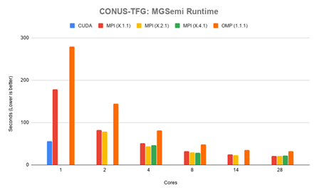
the 14.2.1 con guration, spending 20.75 seconds in the function. OpenMP performed slower than all MPI con gurations, spending 31.78 seconds in the function on 28 cores. Both MPI and OpenMP versions saw very little performance gain once 14 cores were in use. Full timing results can be found in can be found in Appendix B Table B.3
4.3.2 CONUS-RU
The CONUS-RUtest case was run in several con gurations for the MPI and OpenMP versions of ParFlow. For MPI the X in the con guration corresponds to total number of MPI processes. For OpenMP the X in the con guration corresponds to OpenMP threads per MPI process. For example an OpenMP con guration of X.4.1 on 28 cores means 4 MPI processes, each with 7 threads. Full timing results for 1 to 28 cores can
be found in Appendix B Table B.4.
Figure 4.4 shows the total runtime for the CONUS-RU test case in seconds. The CUDA version solved the problem domain in 300.48 seconds, and was slower after more than 2 cores were in use. The MPI version performed equally between each of its con gurations with times only varying by 1 to 2 seconds, attributable to system noise and IO. The fastest time for MPI was in the 28.1.1 con guration, solving in 31.80 seconds. The OpenMP version was slower in each con guration, up to 28 cores.
The fastest time for OpenMP was in the X.4.1 con guration with 28 cores in use, solving in 42.11 seconds.
Figure 4.5 shows timing results for NL Function Eval in seconds. The CUDA version was faster than the MPI version until more than one core was in use, spending in 240.40 seconds the function. The MPI version performed equally between all
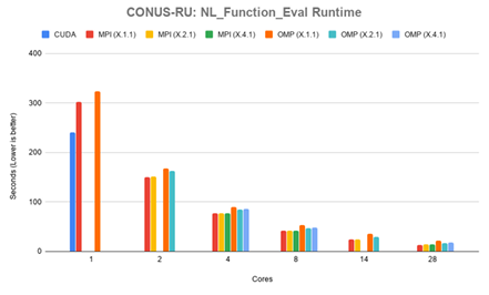
con gurations. The fastest time for MPI was in the 28.1.1 con guration, spending 17.33 seconds in the function. OpenMP was slower than all con gurations up to 8 cores, at which point all con gurations became competitive. The fastest time for OpenMP was 16.60 seconds in the X.2.1 con guration on 28 cores. Full timing results can be found in can be found in Appendix B Table B.5.
Figure 4.6 shows timing results for MGSemi in seconds. The CUDA version was faster than the MPI version until more than 5 cores were in use, spending 7.88 in the function. The MPI version performed equally between all con gurations, with the fastest time of 3.45 seconds in the 28.1.1 con guration. OpenMP was slower than MPI in all con gurations until 18 cores, at which point the X.2.1 con guration became competitive. The fastest time for OpenMP on 28 cores was 3.77 seconds in the X.2.1 con guration. Full timing results can be found in can be found in Appendix B
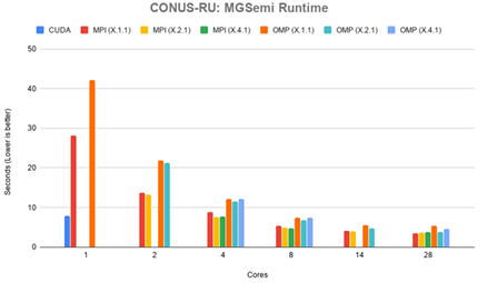
Table B.6.
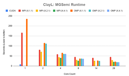
4.3.3 ClayL
The ClayL test case was run in several con gurations for the MPI and OpenMP versions of ParFlow, explained in section 4.3.2. Con gurations presented for the ClayL test case are grouped in terms of total core counts of 1, 2, 4, 8, 14, and 28. Full timing results for 1 to 28 cores can be found in Appendix B Table B.7. Figure 4.7 shows the total runtime results for the ClayL benchmark. In this case, the experimental CUDA version of ParFlow performed best, solving the prob lem domain in 37.30 seconds. The MPI version of ParFlow performed best in the 7.4.1 con guration for 28 cores, solving the problem domain in 59.02 seconds. The experimental OpenMP version solved the problem domain in 63.59 seconds in the
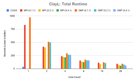
X.4.1 con guration, with each MPI rank using 7 threads. This shows that the CUDA version outperforms MPI in this problem domain, and that the OpenMP version stays competitive when more than 8 cores are used. These results additionally show the impact different domain decompositions have on performance. When the domain is decomposed only along the X axis in a MPI 28.1.1 con guration, performance is 37% slower compared to a 7.4.1 con guration.
Figure 4.8 shows the runtime results for NL Function Eval in ClayL. The CUDA version spent 4.23 seconds of runtime in this function. The MPI version spent 6.66 seconds of runtime in its fastest con guration of 7.4.1. The OpenMP version spent 6.70 of runtime in its fastest con guration of X.4.1 on 28 cores. This corresponds to what was seen in the total runtime results, with CUDA being faster than MPI and Open MP remaining competitive. Full timing results can be found in can be found in
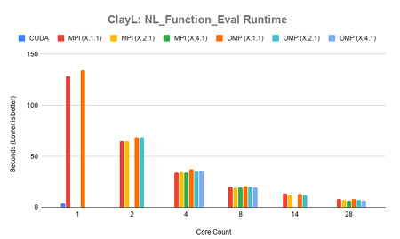
Appendix B Table B.8.
Figure 4.9 shows the runtime results for MGSemi in ClayL. The CUDA version spent 8.06 seconds of runtime in this function. The MPI version spent 20.74 seconds in its fastest con guration of 7x4x1, and OpenMP 19.17 seconds similarly. The CUDA version continues to perform better than MPI. The OpenMP version outperforms the MPI version in certain con gurations. With X.1.1 con gurations OpenMP performed faster than MPI more than 4 cores were in use, and faster in X.2.1 con gurations when at least 14 cores were in use. The X.4.1 con guration became competitive when 20 or more cores were in use. Full timing results can be found in can be found in Appendix B Table B.9.
4.3.4 Summary
The results of this performance study indicate there is potential for improved on-node shared memory parallelism with the experimental OpenMP and CUDA versions of ParFlow. This study highlights the di erent performance characteristics of di erent problem domains. Domain decomposition a ects memory layout and memory access patterns, which can have signi cant e ect on performance results as seen in the ClayL test case. For total runtimes, we see a mix of improved performance and competitive performance for the di erent versions. In the ClayL test case, the CUDA version of ParFlow is faster than the MPI version in its fastest con guration on 28 cores. The Open M Pversion remains competitive with the MPI version when at least 14 cores are in use. The CONUS-RU test case shows the CUDA version is slower once more than one core is in use, and that the OpenMP version is competitive up to 8 cores. In the CONUS-TFGcase, both the CUDAandOpenMPversions of ParFlow are slower than the MPI version. Examining parallel regions to account for KINSOL performance shows strong potential for improved performance using CUDA and OpenMP, and indicate there is room for improvement in these experimental builds. This highlights the importance of a varied suite of test cases when performing benchmarks in a scientific application.
CHAPTER 5
RELATED WORK
Domain Speci c Languages are frequently used in scienti c applications. Typically, they are presented as application-independent libraries or frameworks. Di erent DSLs target di erent use cases, but have a shared interest in architecture portability and performance. DSLs are often used to capture iteration scheduling, applying parallel frameworks, and managing architecture speci c details. The following sections present several related domain speci c languages, grouped by categories of features they encapsulate.
The eDSLabstractions presented in this work focus on boundary condition computations. They are generalizable to other scienti c applications, and are demonstrated in the ParFlow application with no external library or compiler dependencies. Particular emphasis was placed on lifting scienti c computations from the existing code and inserting them into the new eDSL, with minimal rewrites. This is in contrast to most other DSL frameworks, which often require signi cant rewriting of computations.
5.1 Iteration Scheduling
Domain speci c languages are frequently used to abstract and automatically manage iteration domain scheduling. Frameworks such as STELLA [18], Tiramisu [6],
CHOMBO [28], and Intel Thread Building Blocks [26, 33] all provide interfaces for domain scientists to automatically schedule their computations.
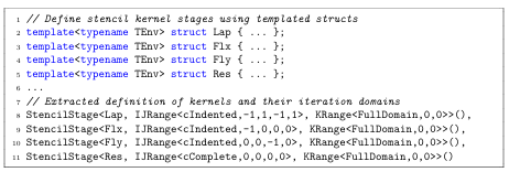
Abstracting loop scheduling removes the need for programmers to directly manage optimizations such as loop fusion or tiling. A programmer can instead specify the domain for a given computation or set of computations and have the DSL generate applicable code. An example of this in the STELLA framework can be seen in Figure 5.1. STELLA was developed for the COSMO [2] scienti c application, used in regional climate modelling. STELLA decomposes stencil computations into a set of building blocks. Each stage of the computation is de ned as a C++ templated data structure. These stages are then combined in the form of a recipe . Each Stencil Stage entry contains the appropriate stencil computation as well as its iteration domain. The iteration domain in STELLA is split into the XY axis and the Z axis, or IJRange and KRange respectively.
This separation of iteration scheduling from the computations allows for backend optimizations to be applied transparently to the programmer [4]. Loop iterations for each stencil entry can be fused, tiled, or have other optimizations applied without obfuscating key computations.
5.2 GPU Parallelization
Di erent target architectures have di erent optimal scheduling patterns, especially in the context of parallel computing. For instance a GPU accelerator may see better parallel performance by ordering storage in a k > j > i fashion, compared to a more typical layout of CPU iterations in a i > j > k order. Storage layout directly a ects memory access patterns. As processors have become faster, memory has increasingly become the bottleneck in performance. Abstracting scheduling and storage is then crucial to enabling performance portable parallel implementations. STELLA, Tiramisu, Accelerate [12], AMReX [48], and ArrayFire [22] support GPU parallelism in their DSL implementations. STELLA o ers two backends for its DSL, a CPU-based OpenMP backend and a CUDA based GPU backend. The frame work allows for either backend to be selected. Storage is automatically rearranged by STELLA depending on this choice, optimizing memory access patterns for the selected architecture at compile time.
Tiramisu and AMReX also o er GPU compute support, but require more input from the programmer. Di erent storage choices must be explicitly stated, as opposed to STELLAs approach of specifying architecture type. Similarly iteration and loop transformations must be stated by the programmer. Accelerate and Array Fire are both GPU-compute speci c DSL extensions, with Accelerate being tailored to Haskell vector computations and Array Fire being a general-purpose API for the C, C++, Python, and Fortr an languages.
5.3 Separation of Computations
A major part of a domain speci c language is the separation of computations from their implementation details. Iteration scheduling, memory and storage management, and other programming concerns must be moved away from the mathematical computations. This allows for parallelism [4] and other optimizations to be applied transparently to computational scientists.
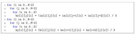
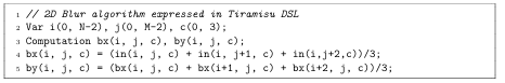
This separation requires careful design, and often introduces a level of code complexity itself. Domain speci c languages are most often presented in the form of a forward-facing API. This may result in computations needing to be reformulated to match the API. An example of a 2D blur algorithm used in image processing can be seen in Figure 5.2. Translating this into the Tiramisu DSL requires a complete rewrite of the computations. This can be seen in Figure 5.3. Tiramisu requires computational
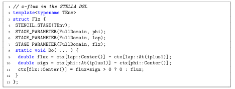
scientists to reformulate computations into purely functional expressions. These expressions are fed into the Tiramisu polyhedral compiler, and an optimized algorithm is produced. STELLA requires similar rewriting of computations. An example of a 4th order ux smoothing in the X direction written in the STELLA DSL can be seen in Figure 5.4. STELLA discretizes stages of the computation, and computational scientists assemble the full formulation as a recipe, as described in Section 5.1. Rewriting of computations is prohibitively expensive. As codebases become larger infrastructure becomes more complex. This causes implementation issues to rise quickly, potentially requiring additional rewriting of the program structure to t a particular DSL. The abstractions in this work were designed with this in mind. The front-end API was designed rst, speci cally to minimize any rewriting of computations. Computations require little to no rewrites in the presented work, able to be lifted directly from the existing code and placed in the proposed eDSL. There is a tradeo to this approach in that the backend becomes more complex to adapt to different hardware architectures, but bene ts computational scientist productivity more directly.
5.4 Enforcing DSL Usage
DSLs provide abstractions for common computational idioms. Complex looping structures, such as Octree navigation, o er performance bene ts. A DSL can en capsulate these looping structures into more easily managed interfaces, improving computational scientist productivity. Mixing non-DSL code, or exposed code, such as explicit loops or conditional branching, degrades the bene ts of a DSL. A DSL must encapsulate as much computation as possible, providing full coverage of the necessary sections of code. It is thus highly desirable for a DSL to be designed in such a way that it is either di cult, inconvenient, or less sensible to write exposed code intermixed with the DSL. The more computational scientists can stay within DSL abstractions, the greater impact they can produce. Proto [34] is a meta-DSL provided as a library. The goal of Proto is to provide a way to write an eDSL utilizng a Backus-Naur style grammar.
This is accomplished through C++ meta-templating features. Approaching the construction of an eDSL in this manner means that stepping outside of DSL abstractions e ectively requires writing in a completely different language. Delite [46, 9] is a framework embedded in the Scala programming language. A set of common components is provided through the framework, such as parallel loops, map functions, ltering, and reductions. Meta programming is leveraged to emit intermediate representation code for di erent languages, such as C or C++. Delite was designed with the intent of being able to write other, more speci c DSL libraries, such as Forge [47] or OptiML [11]. Forge aims to provide a declarative, high-performance DSL for parallel computing. OptiML aims to provide a DSL for machine learning, and provide GPU compute portability. By leveraging Scala in this
manner Delite helps to fully encapsulate computations, as well as provide a strong basis for writing other more speci c DSLs. RDL[45] is a contract-based DSL for the Ruby programming language. Contracts are implemented as a layer on top of di erent functions and objects. If a developer attempts to perform some computation that violates a speci ed contracts, compile time checks will emit errors and prevent the program from building. This ensures that developers stay within the context of the DSL and its features, and provides a layer to ensure validity of the program.
CHAPTER 6
CONCLUSIONS
This thesis presents abstractions for boundary condition computations, demonstrated in the ParFlow application and implemented as an eDSL with no external dependencies. The abstractions are generalizable to iterative solvers that are frequently used in scientific applications, and are demonstrated in the ParFlow application. These
abstractions have directly improved computational scientists productivity, enabling new boundary conditions to be successfully added. Additionally, the abstractions enable architecture portability. An experimental OpenMP version of ParFlow was implemented using these abstractions, and enable the required exibility to unify the experimental CUDA version of ParFlow provided by the Juelich Research Center in Germany.
Aperformance study was conducted on the experimental builds of ParFlow. This study helps indicate what target architectures are worth exploring further. The CUDA version of ParFlow is shown to be faster than the MPI version in certain domains and con gurations. The OpenMP version of ParFlow is shown to be competitive with the MPI version in certain con gurations. The di ering results showcase the complex nature of real world scienti c applications, and highlights the need for performance metrics to be established when optimizing applications and porting to new hardware.
REFERENCES
[1] TOP500 Supercomputers List- June 2019.
[2] Cosmo: Regional climate modeling, cited August 2019.
[3] Mark Adams, Peter O Schwartz, Hans Johansen, Phillip Colella, Terry J Ligocki, Dan Martin, ND Keen, Dan Graves, D Modiano, Brian Van Straalen, et al. Chombo software package for amr applications-design document. Technical report, 2015.
[4] Todd A. Anderson, Hai Liu, Lindsey Kuper, Ehsan Totoni, Jan Vitek, and Tatiana Shpeisman. Parallelizing Julia with a Non-Invasive DSL (Artifact). Dagstuhl Artifacts Series, 3(2):7:17:2, 2017.
[5] Steven F. Ashby and Robert D. Falgout. A parallel multigrid preconditioned conjugate gradient algorithm for groundwater ow simulations. Nuclear Science and Engineering, 124(1):145159, 1996.
[6] Riyadh Baghdadi, Jessica Ray, Malek Ben Romdhane, Emanuele Del Sozzo, Abdurrahman Akkas, Yunming Zhang, Patricia Suriana, Shoaib Kamil, and Saman Amarasinghe. Tiramisu: A polyhedral compiler for expressing fast and portable code. In Proceedings of the 2019 IEEE/ACM International Symposium on Code Generation and Optimization, CGO 2019, pages 193205, Piscataway, NJ, USA, 2019. IEEE Press.
[7] I. J. Bertolacci, M. M. Strout, S. Guzik, J. Riley, and C. Olschanowsky. Identifying and scheduling loop chains using directives. In 2016 Third Workshop on Accelerator Programming Using Directives (WACCPD), pages 5767, Nov 2016.
[8] I. J. Bertolacci, M. M. Strout, J. Riley, S.M.J. Guzi, E. C. Davis, and C Olschanowsky. Using the loop chain abstraction to schedule across loops in existing code. In Int. J. High Performance Computing and Networking, volume 13, pages 86104, 2019.
[9] K. J. Brown, A. K. Sujeeth, H. J. Lee, T. Rompf, H. Cha , M. Odersky, and K. Olukotun. A heterogeneous parallel framework for domain-speci c languages. In 2011 International Conference on Parallel Architectures and Compilation Techniques, pages 89100, Oct 2011.
[10] Donna A. Calhoun and Carsten Burstedde. Forestclaw: A parallel algorithm for patch-based adaptive mesh re nement on a forest of quadtrees. CoRR, abs/1703.03116, 2017.
[11] Hassan Cha , Arvind K. Sujeeth, Kevin J. Brown, HyoukJoong Lee, Anand R. Atreya, and Kunle Olukotun. A domain-speci c approach to heterogeneous parallelism. SIGPLAN Not., 46(8):3546, February 2011.
[12] Manuel M.T. Chakravarty, Gabriele Keller, Sean Lee, Trevor L. McDonell, and Vinod Grover. Accelerating haskell array codes with multicore gpus. In Proceedings of the Sixth Workshop on Declarative Aspects of Multicore Programming, DAMP 11, pages 314, New York, NY, USA, 2011. ACM.
[13] M. Christen, O. Schenk, and H. Burkhart. Patus: A code generation and autotuning framework for parallel iterative stencil computations on modern microarchitectures. In 2011 IEEE International Parallel Distributed Processing Symposium, pages 676 687, May 2011.
[14] Eddie C. Davis, Michelle Mills Strout, and Catherine Olschanowsky. Trans forming loop chains via macro data ow graphs. In Proceedings of the 2018 International Symposium on Code Generation and Optimization, CGO 2018, pages 265277, New York, NY, USA, 2018. ACM.
[15] Jose Fonseca. gprof2dot.
[16] Markus Geimer, Felix Wolf, Brian J. N. Wylie, Erika Abraham, Daniel Becker, and Bernd Mohr. The scalasca performance toolset architecture. Concurrency and Computation: Practice and Experience, 22(6):702719, 2010.
[17] Susan L Graham, Peter B Kessler, and Marshall K McKusick. Gprof: A call graph execution pro ler. ACM SIGPLAN Notices, 39(4):4957, 2004.
[18] Tobias Gysi, Carlos Osuna, Oliver Fuhrer, Mauro Bianco, and Thomas C. Schulthess. Stella: A domain-speci c tool for structured grid methods in weather and climate models. In Proceedings of the International Conference for High Performance Computing, Networking, Storage and Analysis, SC 15, pages 41:141:12, New York, NY, USA, 2015. ACM.
[19] Tianyi David Han and Tarek S. Abdelrahman. Reducing branch divergence in GPU programs. In Proceedings of the Fourth Workshop on General Purpose Processing on Graphics Processing Units, GPGPU-4, pages 3:13:8. ACM. event place: Newport Beach, California, USA.
[20] A. Heinecke, M. Klemm, and H. Bungartz. From GPGPU to many-core: Nvidiafermi and intel many integrated core architecture. 14(2):7883.
[21] Alan C Hindmarsh, Peter N Brown, Keith E Grant, Steven L Lee, Radu Serban, Dan E Shumaker, and Carol S Woodward. SUNDIALS: Suite of nonlinear and di erential/algebraic equation solvers. ACM Transactions on Mathematical Software (TOMS), 31(3):363396, 2005.
[22] Chris McClanahan Vishwanath Venugopalakrishnan Krunal Patel John Mel onakos James Malcolm, Pavan Yalamanchili. Array re: a gpu acceleration platform. 8403, 2012.
[23] Jim E. Jones and Carol S. Woodward. Newtonkrylov-multigrid solvers for large scale, highly heterogeneous, variably saturated ow problems. Advances in Water Resources, 24(7):763 774, 2001.
[24] Mandli K., Ahmadia A., Berger M., Calhoun D., George D., Hadjimichael Y., Ketcheson D., Lemoine G., and LeVeque R. Clawpack: building an open source ecosystem for solving hyperbolic pdes. PeerJ Computer Science, 2016.
[25] Ramgopal Kashyap and Pratima Gautam. Fast level set method for segmentation of medical images. In Proceedings of the International Conference on Informatics and Analytics, ICIA-16, pages 20:120:7, New York, NY, USA, 2016. ACM.
[26] W. Kim and M. Voss. Multicore desktop programming with intel threading building blocks. IEEE Software, 28(1):2331, Jan 2011.
[27] Stefan J. Kollet and Reed M. Maxwell. Integrated surface groundwater ow modeling: A free-surface overland ow boundary condition in a parallel ground water ow model. Advances in Water Resources, 29(7):945 958, 2006.
[28] D. T. Graves J.N. Johnson N.D. Keen T. J. Ligocki. D. F. Martin. P.W. McCorquodale D. Modiano. P.O. Schwartz T.D. Sternberg M. Adams, P. Colella and B. Van Straalen. Chombo software package for amr applications design document. Technical report, Lawrence Berkely National Laboratory, 2019.
[29] R. M. Maxwell, L. E. Condon, and S. J. Kollet. A high-resolution simulation of groundwater and surface water over most of the continental us with the integrated hydrologic model par ow v3. Geoscienti c Model Development, 8(3):923937, 2015.
[30] Reed M. Maxwell. A terrain-following grid transform and preconditioner for parallel, large-scale, integrated hydrologic modeling. Advances in Water Resources, 53:109 117, 2013.
[31] Reed M Maxwell. A terrain-following grid transform and preconditioner for parallel, large-scale, integrated hydrologic modeling. Advances in Water Resources, 53:109117, 2013.
[32] Zdzislaw Meglicki, Stephen K. Gray, and Boyana Norris. Multigrid fdtd with chombo. Computer Physics Communications, 176(2):109 120, 2007.
[33] Chris J. Newburn, Byoungro So, Zhenying Liu, Michael McCool, Anwar Ghuloum, Stefanus Du Toit, Zhi Gang Wang, Zhao Hui Du, Yongjian Chen, Gansha Wu, Peng Guo, Zhanglin Liu, and Dan Zhang. Intels array building blocks: A retargetable, dynamic compiler and embedded language. In Proceedings of the 9th Annual IEEE/ACM International Symposium on Code Generation and Optimization, CGO 11, pages 224235, Washington, DC, USA, 2011. IEEE Computer Society.
[34] Eric Niebler. Proto: A compiler construction toolkit for dsels. In Proceedings of the 2007 Symposium on Library-Centric Software Design, LCSD 07, pages 4251, New York, NY, USA, 2007. ACM.
[35] OpenMP Architecture Review Board. OpenMP application program interface version 4.5, 2015.
[36] R. Rabenseifner, G. Hager, and G. Jost. Hybrid mpi/openmp parallel programming on clusters of multi-core smp nodes. In 2009 17th Euromicro International Conference on Parallel, Distributed and Network-based Processing, pages 427 436, Feb 2009.
[37] Shah M. Faizur Rahman, Qing Yi, and Apan Qasem. Understanding stencil code performance on multicore architectures. In Proceedings of the 8th ACM International Conference on Computing Frontiers, CF 11, New York, NY, USA, 2011. Association for Computing Machinery.
[38] et al Reed M. Maxwell. Hydroframe: A national community hydrologic modeling framework for scienti c discovery, cited August 2019.
[39] Lakshminarayanan Renganarayanan, Daegon Kim, Michelle Mills Strout, and Sanjay Rajopadhye. Parameterized loop tiling. ACM Trans. Program. Lang. Syst., 34(1):3:13:41, May 2012.
[40] Lorenzo Adolph Richards. Capillary conduction of liquids through porous mediums. Physics, 1(5):318333, 1931.
[41] Gerhard Wellein Rolf Rabenseifner. Communication and optimization aspects of parallel programming models on hybrid architectures.
[42] Nikolay Sakharnykh. Everything you need to know about uni ed memory, 2018.
[43] J. Sartori and R. Kumar. Branch and data herding: Reducing control and memory divergence for error-tolerant GPU applications. 15(2):279290.
[44] Kyle Shannon. bsurc/r2-doi: 1.0.17, November 2018.
[45] T. Stephen Strickland, Brianna M. Ren, and Je rey S. Foster. Contracts for domain-speci c languages in ruby. SIGPLAN Not., 50(2):2334, October 2014.
[46] Arvind K. Sujeeth, Kevin J. Brown, Hyoukjoong Lee, Tiark Rompf, Hassan Cha , Martin Odersky, and Kunle Olukotun. Delite: A compiler architecture for performance-oriented embedded domain-speci c languages. ACM Trans. Embed. Comput. Syst., 13(4s):134:1134:25, April 2014.
[47] Arvind K. Sujeeth, Austin Gibbons, Kevin J. Brown, HyoukJoong Lee, Tiark Rompf, Martin Odersky, and Kunle Olukotun. Forge: Generating a high performance dsl implementation from a declarative speci cation. SIGPLAN Not., 49(3):145154, October 2013.
[48] Weiqun Zhang, Ann Almgren, Vince Beckner, John Bell, Johannes Blaschke, Cy Chan, Marcus Day, Brian Friesen, Kevin Gott, Daniel Graves, Max Katz, Andrew Myers, Tan Nguyen, Andrew Nonaka, Michele Rosso, Samuel Williams, and Michael Zingale. Amrex: a framework for block-structured adaptive mesh re nement. Journal of Open Source Software, 4(37):1370, 5 2019.
APPENDIX A
REPRODUCIBILITY
This appendix covers steps to reproduce the results in this work. See Appendix B for the full timing results of the performance study. ParFlow was compiled using the basic instructions found in the users manual, with the following CMAKE command

For the CUDA version, the additional ag was enabled:
![]()
And similarly for the OpenMP version the additional ag was enabled:
![]()
Libraries used were: GCC 7.2.0, MPICH 3.2.1, CMake 3.12, TCL 8.5, and CUDA 10.1. When compiling on R2, it may be necessary to explicitly tell CMake to use mpicc and mpicxx as the C and CXX compilers in order to avoid a linking error.
This is an environmental issue, and can be resolved by exporting the CC and CXX variables to point directly at mpicc and mpicxx. The MPI version can be found at the following github repo and commit hash
https://github.com/hydroframe/ParFlow_PerfTeam/tree/pf_newbc Hash: 983aadd45b83cce9272b971a7bbb960a7b602b92 The OpenMP version can be found at the following github repo and commit hash https://github.com/hydroframe/ParFlow_PerfTeam/tree/pf_omp_newbc
Hash: 237198f999f190a41cc822b0166bdd973d8f02a2
The CUDA version can be found at the following github repo and commit hash
https://github.com/hokkanen/parflow/tree/CUDA
Hash: a7d788deaefa285c31c9ab90accbbe6dca9b412f
APPENDIX B
DATA
Appendix B contains full timing results of the performance study.
TableB.1: Total Run time in seconds for CONUS-TFG

TableB.2: CONUS- TFG: Run time in seconds for NL Function Eval

TableB.3: CONUS-TFG: Run time in seconds for MGSemi

TableB.4:Total Run time for CONUS-R Uin seconds

TableB.5: Runtime for NL Function Eval in CONUS-RU(in seconds)

TableB.6: Runtime for MG Semi in CONUS-RU(in seconds)

TableB.7: Total Runtime for Clay Lin seconds

TableB.8: Runtime for NL Function Eval in ClayL(in seconds)

TableB.9: Runtime for MG Semi in ClayL(in seconds)


